Metrics
Metrics aggregate, store, and compute statistics for time-based data.
- Names
- Types
- Dimensions
- Periods
- Statistics
- Retention
- Eventual consistency
- Built-in metrics
- Using metrics in reports
- Using metrics in automations
Names
Each metric has a unique, namespaced identifier (e.g. cerb.workers.active) using dot-notation.
The cerb. prefix is reserved for built-in metrics. You can create your metrics with any other prefix.
By convention, the prefix is most often a domain name you own in reverse order (e.g. com.example.metric.name) to ensure global uniqueness. This makes it easier to combine and share metrics across multiple Cerb environments.
Types
Each metric is one of these types:
| Type | Description |
|---|---|
counter |
A value that increments over time (e.g. automation invocations and durations, new tickets received, failed worker logins) |
gauge |
A direct reading of a value at a given time (e.g. CPU load, active workers, open tickets per bucket, assignments per worker) |
Metric types automatically configure reporting and visualizations, but do not affect how the underlying data samples are stored.
Dimensions
A single metric may be further partitioned by adding up to three optional key/value pairs called dimensions to its samples. The possible dimensions are defined ahead of time on the metric, but can be provided in any order with the samples.
A dimension is of one of the following types:
| Type | Description of value |
|---|---|
extension |
A platform extension ID (e.g. record type) |
number |
A whole number |
record |
An ID of a given record type |
text |
Any textual value |
Each unique combination of metric and dimensions can function as a separate metric.
For example, the cerb.tickets.open.elapsed metric has dimensions for group_id and bucket_id.
When just querying the cerb.tickets.open.elapsed metric, the results will combine all dimensions together. The metric could also be queried for any combination of groups, or for a specific set of buckets. These dimensions could be reported independently or compared to each other.
For performance, all text-based dimension values are mapped to a corresponding integer value. This requires much less storage and enables fast lookups and filtering. The number and record types are more efficient because they can be directly stored and used as integers, without bloating the mapping.
Periods
Metrics aggregate samples at three levels of detail called periods.
| Period | Count per day |
|---|---|
| 5 minutes | 288 |
| Hourly | 24 |
| Daily | 1 |
These base periods can be further combined in reports: 15 mins, 2 hours, 12 hours, weeks, months, quarters, and years.
A fast-moving metric can be charted every 5 minutes over the past few hours; while a longer-term trend can be visualized daily over the past few months.
The statistics within these periods are precalculated for efficient reporting. This is much faster than reporting based on the samples themselves.
Why not also store months and years?
The main reason is we're more likely to overflow the maximum value for sum over larger periods. By combining smaller periods we can scale the units (e.g. bytes to gigabytes, seconds to hours) as the time range increases.
Statistics
Samples collected within the same period are aggregated into a statistic set with the following values:
| Statistic | Description |
|---|---|
samples |
The number of samples collected for this period |
sum |
The sum of all sample values for this period |
min |
The smallest sample value observed this period |
max |
The largest sample value observed this period |
average |
The average sample value observed this period |
The average is not actually stored, since it's easily computed as the sum divided by samples.
This allows new samples to be continuously added during the same period.
For instance, a counter that increases by +1 for 1,000 events within the same 5-minute period would only store a single statistics set rather than one thousand individual samples. It would look like:
| samples | 1000 |
| sum | 1000 |
| min | 1 |
| max | 1 |
| average | 1 |
For a counter that increments by +1, the most useful statistic is sum. The min, max, and average of the samples are always 1.
However, counters can also increase by values other than +1. We might have a counter for the time automations spend executing in milliseconds. In that case, the min (fastest execution time in the period), max (slowest execution time in the period), and average (average execution time in the period) would be useful in addition to the overall sum (total execution time in the period).
Similarly, a gauge that takes a reading every 5 minutes would store a single statistics set per hour rather than 12 individual samples.
Let's assume a gauge measured the current number of open tickets every 15 minutes for an hour. It took these readings:
| 45 |
| 49 |
| 41 |
| 38 |
It would store this hourly statistics set:
| samples | 4 |
| sum | 174 |
| min | 38 |
| max | 49 |
| average | 43.5 |
For a gauge, the average, min, and max statistics are the most useful. The sum is almost never useful directly, but it is used with samples to compute the average.
From these results, we could report that the average number of open tickets during this hour was 43.5, with a high of 49 and a low of 38. If we sampled 3x more often (every 5 minutes instead of 15 minutes) we'd still only have a single statistics set for the hour, but we'd have a higher samples and sum value, and the min, max, and average would be more precise.
The daily statistics set for this gauge would record the min, max, and average for the entire day.
The ideal frequency of measuring samples for a gauge depends on how that metric will be used. Something that changes infrequently, like the size of your Cerb database in gigabytes, could be measured once daily, weekly, or even monthly. There would be no value in sampling that every minute.
The more expensive a reading, the less often it should be sampled. When you create a report with sparse samples on a gauge metric, Cerb will fill in the missing samples by repeating the most recent prior value until the next value.
Retention
Keeping the data for high-frequency periods has a cost. There are (288) 5-minute periods per standard day, which could produce up to (105,120) 5-minute periods per standard year. That's further multiplied by the distinct dimensions per metric. More storage and processing power is required with each metric and dimension you add.
The length of time that data is kept is called its retention.
Generally, the farther back you look in time, the less useful the smaller periods are (e.g. 5 minutes).
If you're reporting on data from a year ago, it probably doesn't matter what a metric's average value was for a specific 5-minute period. For prior period comparisons, it's often most useful to compare with larger periods like days, weeks, months, or years.
Cerb automatically removes aging high-frequency data to keep storage and processing costs lower.
The default retention time per period is:
| Period | Retention |
|---|---|
| 5 minutes | 24 hours |
| Hourly | 2 weeks |
| Daily | forever |
The 5-minute period is a "sliding window" over the trailing 24 hours. When a new 5-minute period starts, the oldest period (crossing 24 hours in age) is removed. This maintains a constant set of (288) most recent 5-minute periods per metric.
Eventual consistency
When multiple samples are collected in a short time period, with the same metric and dimensions, they are combined into a single statistics set. This single set is then pushed into a background queue for processing.
With this approach, you can efficiently collect samples at very high volumes without sacrificing performance.
For instance, the email parser is not delayed by sampling many metrics for every new inbound message (e.g. language, region, org, industry, classification, intent, etc).
Because samples are processed in the background, the most recent data may not show up on charts for a few minutes.
Built-in metrics
These metrics are managed automatically by Cerb:
| Metric | Description |
|---|---|
| cerb.automation.duration | How long automations are executed. Dimensions: automation_id and trigger. |
| cerb.automation.invocations | How often automations are executed. Dimensions: automation_id, trigger, exit_state. |
| cerb.behavior.duration | How long behaviors are executed. Dimensions: behavior_id and event. |
| cerb.behavior.invocations | How often behaviors are executed. Dimensions: behavior_id and event. |
| cerb.mail.routing.rule.matches | Mail routing rule usage over time. Dimensions: rule_id (by ruleset record), rule_key (by rule), and node_key (by condition). |
| cerb.mail.transport.deliveries | How many successful messages are sent through a mail transport. Dimensions: transport_id and sender_id (email address). |
| cerb.mail.transport.failures | How many unsuccessful messages are attempted through a mail transport. Dimensions: transport_id and sender_id (email address). |
| cerb.record.search | How often each worker searches for a given record type. Dimensions: record_type and worker_id. |
| cerb.snippet.uses | Snippet usage over time by worker. Dimensions: snippet_id and worker_id. This replaces the snippet_use_history table but imports its data. |
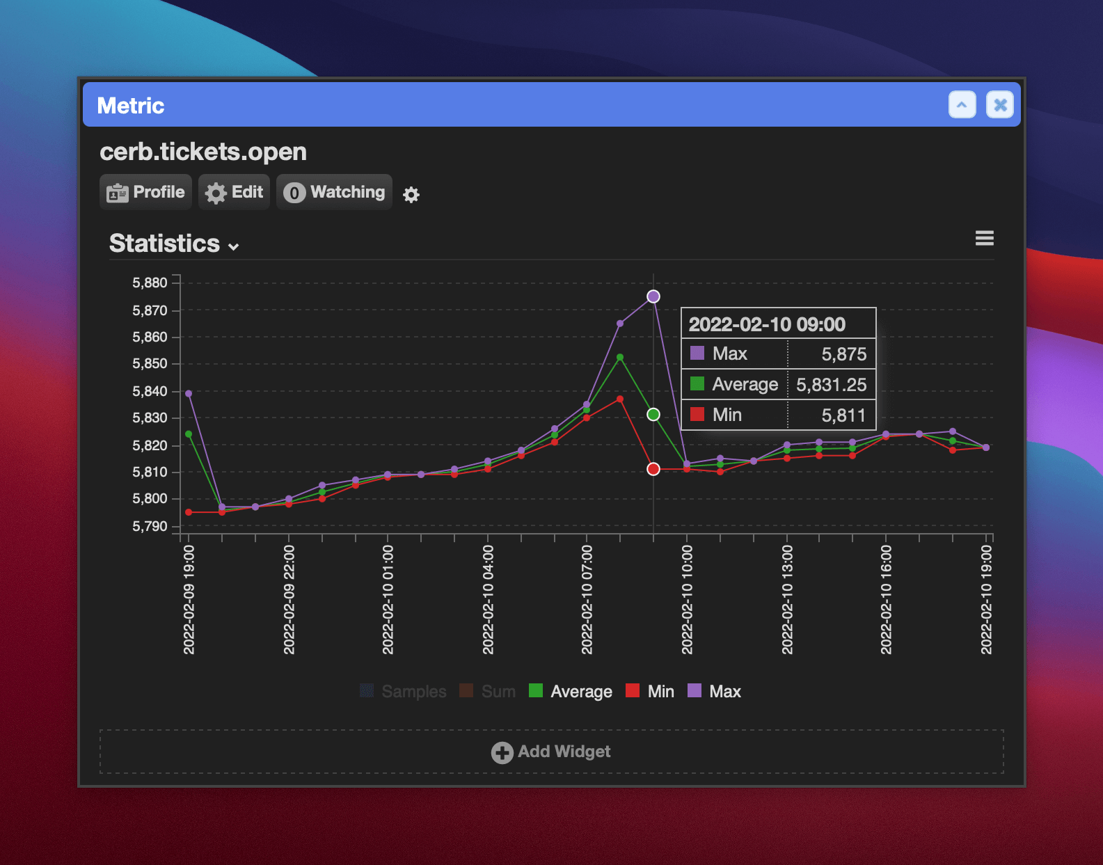
| cerb.tickets.open | Open ticket counts over time by group and bucket. Dimensions: group_id and bucket_id. The metric is sampled every 15 minutes. |
| cerb.tickets.open.elapsed | How long tickets spent in the open status by group and bucket. Dimensions: group_id and bucket_id. The metric is sampled when an open ticket is moved to a new group/bucket, or an open ticket transitions to a non-open status. |
| cerb.webhook.invocations | How often webhooks are executed. Dimensions: webhook_id and client_ip. |
| cerb.workers.active | Seat usage by workers. Dimensions: worker_id. |
Using metrics in reports
Metrics statistics can be retrieved with metrics.timeseries data queries.
Using metrics in automations
You can record samples on a metric from automations with the metric.increment command.